Why Engineers Who Deeply Understand AI Architecture Must Master This Diagram¶

The Geometric Skeleton Beneath the Operator¶

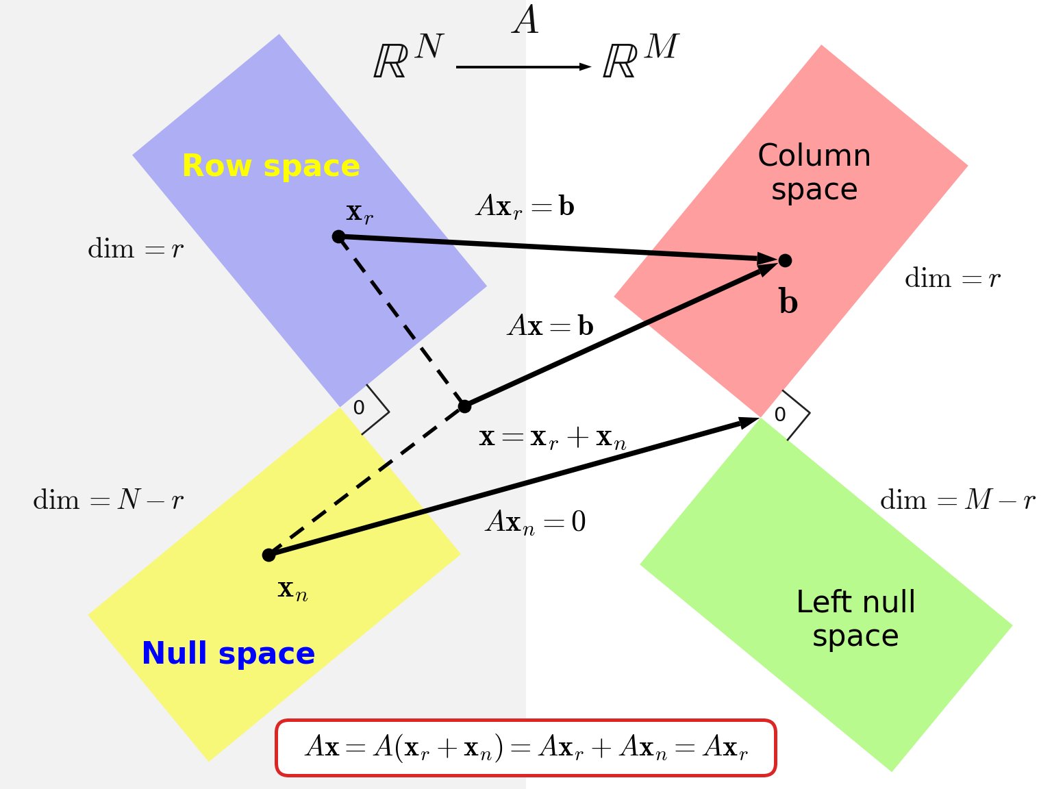
While polishing Chapter 3 (Subspaces and Orthogonality) of Mathematics for AI & ML today, I redrew the classic Big Picture from my linear algebra professor at MIT, Gilbert Strang: the action of a matrix $A$ on the four fundamental subspaces.

Drawing this diagram brought back a flood of memories.

I had actually taken linear algebra as a college sophomore, memorizing formulas for eigenvalues and determinants and scoring a 92, but my head was filled with ungrounded rules. To this day I still hold a grudge against the Chinese translation for determinant (行列式)—it sounds like an algebraic expression or formula, yet it simply evaluates to a scalar value.

I stumbled through the door with that fog in my head. It was only later, sitting in Professor Strang's classroom at MIT, that I heard him take space apart from a completely different perspective. When he introduced the Four Fundamental Subspaces, I found it fascinating, yet I couldn't help wondering: What is this actually good for? Our college textbooks back home had never even mentioned them.

He spoke steadily, never rushing. Whenever he reached a pivotal step in a derivation, he would pause, fold his arms across his chest, stand in thought, and then turn to ask us: "Why?" During a break, I went up to ask about the geometric intuition behind an algebraic problem. He smiled, sketched a few simple strokes on the blackboard, and everything clicked at once.

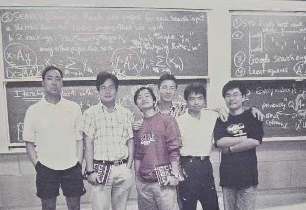
That door opened for me then. Mathematics ceased to be a pile of dry formulas; it became a language for describing geometric structure and transformation.

I only learned much later that Professor Strang was the one who originally introduced the Four Fundamental Subspaces into modern linear algebra education. Wow—how incredibly lucky I was to have been sitting in his classroom!

Years later, when I wrote Mathematics for AI & ML, it was very much to follow in my teacher's footsteps—passing that same intuitive geometric foundation on to others.

Engineers just entering the field often view modern AI as little more than matrix multiplication and API wrapping: call nn.Linear, write y = model(x), let automatic differentiation compute gradients, and let AdamW optimize the loss. Why bother with dimension theorems, direct sums, and null spaces?—much like I sat in that MIT classroom wondering: What is this actually good for?

Yet when a large language model collapses on a downstream task, when fine-tuning ruins general capabilities, when imperceptible adversarial noise fools a vision classifier, or when one ponders why a 70B-parameter model can learn new behaviors with a rank-8 LoRA adapter—code alone offers no explanation.

The answer is entirely encoded in the picture my teacher drew for us years ago.

Decoding the Big Picture¶

Mathematically, given any real matrix $A \in \mathbb{R}^{M \times N}$ representing a linear mapping layer in a neural network, the universe of inputs and outputs splits into four fundamental building blocks:

1. The Input Space $\mathbb{R}^N$: Signal vs. Silence¶

The input space partitions cleanly into two mutually orthogonal complements:
- Row space $C(A^\top)$: Dimension $r$ (the rank). These are the effective input directions that directly determine the output.
- Null space $N(A)$: Dimension $N - r$. Any vector lying here is extinguished by $A$ into the zero vector $\mathbf{0}$.

By the orthogonal direct sum decomposition, every input vector $\mathbf{x} \in \mathbb{R}^N$ decomposes uniquely and cleanly into:

2. The Output Space $\mathbb{R}^M$: Reachable vs. Impossible¶

The output space splits symmetrically into two orthogonal counterparts:
- Column space $C(A)$: Dimension $r$. This represents the entire reachable domain of outputs $A$ can possibly produce.
- Left null space $N(A^\top)$: Dimension $M - r$. This is the space of directions $A$ can never reach, capturing irrecoverable errors and residuals.

3. The Action of $A$¶

When $A$ multiplies an arbitrary input $\mathbf{x}$, the decomposition reveals its true nature:

$A$ acts as a pure information filter:
It erases the null-space component $\mathbf{x}_n$ entirely, while mapping the row-space component $\mathbf{x}_r$ one-to-one and invertibly onto the target vector $\mathbf{b}$ in the column space.

Five Geometric Insights Connecting to Modern AI Architecture¶

Once the orthogonal geometry of these four fundamental subspaces takes root in your intuition, empirical phenomena across modern deep learning find clear theoretical anchors.

1. LoRA: Null-Space Invariance of Low-Rank Adapters¶

In mainstream open-source foundation models (such as LLaMA and Qwen), attention and feed-forward layers span thousands of dimensions ($d = 4096$ or $8192$). Full fine-tuning requires updating billions of weights in $\Delta W \in \mathbb{R}^{d \times d}$.

Low-Rank Adaptation (LoRA) posits that downstream task adaptation has a very low intrinsic rank, constraining the weight update explicitly as a factored linear operator:

Examining this linear update operator $\Delta W$ through Strang's lens:
- Row space $C((\Delta W)^\top) = C(A^\top)$: Dimension at most $r$ (e.g., $r = 8$ or $16$). Only input representations $\mathbf{x}_r$ with non-zero projection onto this narrow row space trigger an adaptation response: $\Delta W \mathbf{x}_r = B(A\mathbf{x}_r)$.
- Algebraic null space $N(\Delta W) = N(A)$: Dimension at least $d - r$. For the vast majority of input directions $\mathbf{x}_n \in N(A)$ orthogonal to the adapter's row space, the update evaluates strictly to zero: $\Delta W \mathbf{x}_n = \mathbf{0}$.
- Along these high-dimensional null-space directions, the total layer output remains $W_{\text{new}}\mathbf{x}_n = (W_0 + \Delta W)\mathbf{x}_n = W_0\mathbf{x}_n$, entirely governed by the pre-trained base representations. Geometrically, this explains why low-rank adaptation can steer task-specific behaviors while exercising minimal interference across the broader representation space.

2. The Generalization Miracle of Overparameterization: Implicit Regularization in Gradient Flow¶

Classical statistics cautions that when the parameter count far exceeds the number of data samples ($N \gg M$), severe overfitting is guaranteed.

Yet whether in classical vision networks (tens of millions of parameters fitted to a million images) or in full-parameter fine-tuning of modern LLMs, models operate where parameters vastly outnumber sample constraints. Why do first-order optimizers exhibit strong generalization rather than simply memorizing the training set?

Deep learning theory (specifically the Neural Tangent Kernel, or NTK, and overparameterized regression) provides an elegant answer grounded in subspaces:
- Consider the vector of model predictions across all $M$ training samples: $\mathbf{f}(\mathbf{w}) \in \mathbb{R}^M$. The Jacobian matrix of these predictions with respect to the $N$ parameters, $J(\mathbf{w}) \in \mathbb{R}^{M \times N}$ (where $J_{ij} = \frac{\partial f(\mathbf{x}_i; \mathbf{w})}{\partial w_j}$), is an extremely wide matrix with an immense parameter null space: $\dim(N(J)) = N - M \gg 0$.
- By the chain rule, the gradient of the empirical loss with respect to parameters lies strictly in the row space of the Jacobian: $\nabla_{\mathbf{w}} \mathcal{L} = J(\mathbf{w})^\top \mathbf{e} \in C(J(\mathbf{w})^\top)$.
- In linear models or in the "lazy training" regime of overparameterized networks, $J(\mathbf{w}) \approx J_0$ remains nearly static during training. Starting from near-zero initialization, pure gradient descent accumulates updates solely within the fixed row space $C(J_0^\top)$, never venturing into the unconstrained null space $N(J_0)$.
- Out of the infinitely many interpolating solutions that achieve zero training error, gradient flow automatically converges to the minimum Euclidean norm solution:

• While nonlinear architectures and adaptive optimizers (such as AdamW with coordinate scaling and weight decay) break strict Euclidean subspace invariance, this geometric mechanism—updating along the data-gradient row space while leaving the null space untouched—serves as the foundational theoretical model for implicit regularization.

3. Adversarial Robustness: Energy Dissipation vs. Targeted Stings¶

Why can an imperceptible perturbation $\boldsymbol{\delta}$ fool a vision classifier into catastrophic error, even while the same model tolerates substantial amounts of random Gaussian or sensor noise?

High-dimensional subspace decomposition reveals two entirely different geometric realities:
- Variance dissipation of random noise: Suppose input dimension is $D$ (e.g., a million pixels in high resolution), while decision-sensitive features occupy a low-dimensional subspace of dimension $r \ll D$. When isotropic Gaussian noise $\boldsymbol{\delta}$ is injected, high-dimensional geometry dictates that its energy is evenly distributed across all orthogonal directions. The expected fraction of noise energy falling into the sensitive feature subspace is only $\frac{r}{D} \ll 1$; the vast majority is dissipated harmlessly into the orthogonal complement. This is why high-dimensional models naturally withstand random noise.
- Lossless alignment of adversarial noise: Adversarial attacks like FGSM ($\boldsymbol{\delta} = \epsilon \operatorname{sign}(\nabla_{\mathbf{x}} \mathcal{L})$) exploit the end-to-end loss gradient with respect to the input pixels. Instead of dispersing energy isotropically, backpropagation computes the exact sensitive direction, concentrating the entire perturbation budget into the gradient subspace with zero waste in irrelevant dimensions. Consequently, even an infinitesimal norm suffices to breach the decision boundary.

4. Residuals and Projections: The Bedrock of the Left Null Space¶

While the preceding pillars examine the input side (row space and null space), the output side's left null space $N(X^\top)$ is the matrix foundation of linear projection and estimation error throughout machine learning.

In the classic linear least-squares problem $X\mathbf{w} \approx \mathbf{y}$:
- No matter how one tunes the parameter vector $\mathbf{w}$, model predictions $\hat{\mathbf{y}} = X\mathbf{w}$ can never escape the column space $C(X)$.
- The optimal $L_2$ approximation of the target $\mathbf{y}$ is its orthogonal projection $\hat{\mathbf{y}} = P_{C(X)}\mathbf{y}$. At this optimum, the residual error vector:

drops perpendicularly into the orthogonal complement of the column space—which is precisely the left null space $N(X^\top)$.
- The celebrated normal equation $(X^\top X)\mathbf{w} = X^\top \mathbf{y}$ is nothing more than the statement that the residual is orthogonal to every feature column ($X^\top \mathbf{e} = \mathbf{0}$). From ordinary least squares and PCA to Kalman filtering, the entire architecture of classical estimation rests on this fundamental orthogonal decomposition.

5. Generative Models: From Linear Subspaces to Manifold Tangent Spaces¶

In modern generative modeling—from continuous-time diffusion models to flow matching—this geometric intuition elevates from global linear subspaces to local differential geometry.

The manifold hypothesis posits that natural high-dimensional data (e.g., images in $\mathbb{R}^D$) concentrates on a low-dimensional nonlinear manifold $\mathcal{M}$.
- As Gaussian noise is added during the forward process, the noise cloud obscures the manifold geometry.
- Denoising networks learn the score function $\nabla_{\mathbf{x}_t} \log p_t(\mathbf{x}_t)$; through Tweedie's formula, they guide noisy states back toward the high-density data manifold.
- Although a nonlinear manifold's tangent space $T_{\mathbf{x}}\mathcal{M}$ and normal space rotate from point to point, this reflects the profound extension of Strang's direct sum decomposition:
- The tangent space carries legitimate semantic variance and structure;
- The normal space carries isotropic off-manifold noise.
- The reverse generative process progressively strips away normal-direction noise at each infinitesimal step, constraining trajectory dynamics along the tangent space of the data manifold to reconstruct sharp, coherent samples.

Closing¶

In modern AI engineering, modular frameworks make it easy to treat models as black-box compute graphs.

Yet whether an architecture converges, whether it resists adversarial perturbations, whether it fine-tunes without forgetting, or whether it scales efficiently depends not on code syntax, but on underlying subspace projections and orthogonality.

A matrix is not a grid of numbers; it is a geometric filter of space. That quiet "Why?" Professor Strang asked with arms folded at the blackboard was probing this exact geometric foundation.

The next time you examine an attention matrix, initialize a LoRA adapter, or inspect a diffusion loss curve, picture these four orthogonal planes:

行聚精微见性真，
零消冗浊寂无尘。
列开万象穷所至，
左度残差一念深。

(Row gathers essence where the true signals start,
Null stills the turbid noise to silence apart;
Col spans the boundless worlds reachable in sight,
Left null measures the residual depth into night.)

Understand this diagram from my teacher, and the black box becomes transparent.